Scoring
All scoring functions used in the CrowdCent Challenge can be found in the crowdcent_challenge.scoring module.
Raw Metrics
These metrics measure how well your predictions match the actual outcomes, without considering the meta-model.
Symmetric NDCG@k (symmetric_ndcg_at_k)
One of the key metrics used in some challenges is Symmetric Normalized Discounted Cumulative Gain (Symmetric NDCG@k).
Concept
Normalized Discounted Cumulative Gain (NDCG@k) is a metric used to evaluate how well a model ranks items. It assesses the quality of the top k predictions by:
- Giving higher scores for ranking truly relevant items higher.
- Applying a logarithmic discount to items ranked lower (meaning relevance at rank 1 is more important than relevance at rank 10).
- Normalizing the score by the best possible ranking (IDCG) to get a value between 0 and 1.
However, this commonly used metric only focuses on the top items in a list. In finance, identifying the worst performers (lowest true values) can be just as important as identifying the best.
Our metric of Symmetric NDCG@k addresses this by evaluating ranking performance at both ends of the list:
- Top Performance: It calculates the standard
NDCG@kbased on your predicted scores (y_pred) compared to the actual true values (y_true). This measures how well you identify the items with the highest true values. - Bottom Performance: It calculates another
NDCG@kfocused on the lowest ranks. It does this by:- Inverting both true values and predictions using
1 - valuetransformation - This makes originally low values (close to 0) become high values (close to 1), so standard NDCG rewards finding the originally lowest items
- Calculating
NDCG@kfor how well your lowest predictions match the items with the lowest true values
- Inverting both true values and predictions using
- Averaging: The final
symmetric_ndcg_at_kscore is the simple average of the Top NDCG@k and the Bottom NDCG@k.(NDCG_top + NDCG_bottom) / 2.
Calculation
The Symmetric NDCG@k is calculated as:
- Top NDCG@k: Calculate standard NDCG@k using true values and predicted scores
- Bottom NDCG@k: Invert both true values and predictions using
1 - value, then calculate NDCG@k - Final Score: Average of top and bottom NDCG@k scores:
(NDCG_top + NDCG_bottom) / 2
The standard NDCG formula includes:
- DCG@k = Σ(relevance_i / log₂(i+1)) for i=1 to k
- IDCG@k = DCG@k for ideal ranking
- NDCG@k = DCG@k / IDCG@k
Interpretation
Notably, Symmetric NDCG@k does not give 0.5 for random predictions, but ~0.55 for our default k=40. Understanding the random baseline is crucial for interpreting your scores.
- NDCG@k = 1: perfect performance at identifying both the top k best and bottom k worst items according to their true values.
- NDCG@k = 0.55: random guessing.
- NDCG@k = 0: no overlap with top k or bottom k.
How k Affects the Random Baseline:
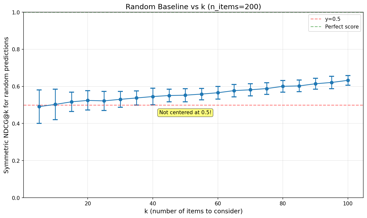
Key insights:
- Random baseline starts near 0.5 for small k and increases monotonically
- For Hyperliquid (k=40, n≈170-200), random predictions score ~0.55
Usage
from crowdcent_challenge.scoring import symmetric_ndcg_at_k
import numpy as np

# Example data
y_true = np.array([0.1, 0.2, 0.9, 0.3, 0.7])
y_pred = np.array([0.2, 0.1, 0.8, 0.4, 0.6])
k = 3

score = symmetric_ndcg_at_k(y_true, y_pred, k)
This metric provides a more holistic view of ranking performance when both high and low extremes are important.
Spearman Correlation (spearman_correlation)
Spearman's rank correlation coefficient is a non-parametric measure of rank correlation that assesses how well the relationship between two variables can be described using a monotonic function.
Concept
In the context of ranking challenges, Spearman correlation measures how well your predicted rankings align with the true rankings. Unlike Pearson correlation (which measures linear relationships), Spearman correlation:
- Works with ranks: It converts both predicted and true values to ranks before computing correlation
- Captures monotonic relationships: Perfect Spearman correlation (±1) means perfect monotonic relationship, even if not linear
- Robust to outliers: Since it uses ranks rather than raw values, extreme values have less influence
Calculation
The Spearman correlation coefficient (ρ) is calculated as:
- First, convert both
y_trueandy_predto ranks - Then calculate the Pearson correlation coefficient on these ranks
- Formula: ρ = 1 - (6 × Σd²) / (n × (n² - 1)), where d is the difference between paired ranks
Interpretation
- ρ = 1: Perfect positive correlation (your rankings perfectly match the true rankings)
- ρ = 0: No correlation (your rankings are unrelated to the true rankings)
- ρ = -1: Perfect negative correlation (your rankings are exactly reversed)
Usage
from crowdcent_challenge.scoring import spearman_correlation
import numpy as np

# Example data
y_true = np.array([1.0, 0.5, 0.3, 0.2, 0.1])  # True values (will be ranked)
y_pred = np.array([0.9, 0.6, 0.25, 0.22, 0.05])    # Predicted values (will be ranked)

score = spearman_correlation(y_true, y_pred)
Uniqueness Metrics
In addition to measuring how accurate your predictions are, we also measure how unique they are relative to the meta-model. If everyone submits the same signal, the meta-model gains nothing. Uniqueness metrics quantify the additional value your predictions bring beyond what the crowd already knows.
Uniqueness metrics are only computed when a meta-model is available for the inference period.
All uniqueness scoring functions are in the crowdcent_challenge.scoring module:
from crowdcent_challenge.scoring import (
    neutralize_predictions,
    unique_ndcg,
    unique_spearman,
    corr_to_meta
)
Neutralization (neutralize_predictions)
Concept
Neutralization is the mathematical building block behind uniqueness scoring. It removes the component of your predictions that's explained by the meta-model, leaving only the orthogonal residual -- the part of your signal the meta-model doesn't already capture.
Intuitively: if your predictions are 80% meta + 20% your own alpha, neutralization strips away the 80% and isolates the 20%.
Calculation
The process uses ordinary least-squares regression:
- Regress your predictions against the meta-model predictions (with an intercept)
- Subtract the fitted values from your predictions
- The residual is your unique signal
Interpretation
The residual has zero correlation with the meta-model by construction. Larger residual variance means more unique signal. If your predictions are nearly identical to the meta, the residual will be near-zero noise.
Usage
from crowdcent_challenge.scoring import neutralize_predictions

residual = neutralize_predictions(y_pred=my_preds, meta_pred=meta_preds)
# residual is uncorrelated with meta_preds by construction
Unique NDCG@40 (unique_ndcg)
Concept
Measures whether your unique signal correctly identifies the top and bottom k assets. This combines neutralization and Symmetric NDCG@k: first your predictions are neutralized against the meta-model, then Symmetric NDCG@k is computed between the residual and y_true.
Calculation
- Neutralize
y_predagainstmeta_predusing OLS regression (see Neutralization above) - Compute Symmetric NDCG@k between the residual and
y_true(see Symmetric NDCG@k for details)
Interpretation
- Range: 0 to 1
- ~0.55: Random (same baseline as raw NDCG@40, since the underlying metric is the same)
- > 0.55: Your unique signal has predictive ranking quality at the extremes
Usage
from crowdcent_challenge.scoring import unique_ndcg

score = unique_ndcg(y_true=actuals_10d, y_pred=my_preds_10d, meta_pred=meta_preds_10d, k=40)
Unique Spearman (unique_spearman)
Concept
Measures whether your unique signal has predictive rank correlation with the actual outcomes. This combines neutralization and Spearman correlation in one step: first your predictions are neutralized against the meta-model, then Spearman correlation is computed between the residual and y_true.
Calculation
- Neutralize
y_predagainstmeta_predusing OLS regression (see Neutralization above) - Compute Spearman rank correlation between the residual and
y_true
Interpretation
- Range: -1 to +1
- Positive: Your unique signal adds predictive value beyond the meta
- Zero: Your unique signal is noise
- Negative: Your unique signal is counter-predictive
Values of 0.02-0.05 are meaningful given the noise in financial data.
Usage
from crowdcent_challenge.scoring import unique_spearman

score = unique_spearman(y_true=actuals_10d, y_pred=my_preds_10d, meta_pred=meta_preds_10d)
Correlation to Meta (corr_to_meta)
Concept
Measures how aligned your predictions are with the meta-model using Spearman rank correlation. This is a direct similarity measure -- it tells you how much your signal overlaps with the crowd.
Unlike the other uniqueness metrics, this does not require y_true -- it is purely a comparison between your predictions and the meta-model. Computed separately for each horizon (10d, 30d).
Calculation
Spearman rank correlation between y_pred and meta_pred. Both vectors are converted to ranks, then Pearson correlation is computed on the ranks (see Spearman Correlation above for details).
Interpretation
- +1: Identical to meta (no unique information)
- 0: Orthogonal to meta (maximally differentiated)
- -1: Exact inverse of meta
Lower is more unique
Unlike raw metrics where higher is better, for corr_to_meta a value closer to zero indicates more unique predictions. However, being unique alone isn't enough -- your unique signal also needs to be predictive.